Why a 99% Accurate Test Is Often Wrong

Is 99% accuracy good enough? If you read Part 3 of this series, you saw that Galleri achieves 99.5% specificity, Shield hits 89.6%, and Cologuard Plus reaches 91%. These sound like excellent numbers. But here is the uncomfortable truth: a positive result from a 99% accurate test might mean you have less than a 1% chance of actually being sick.

Companion to the 3-part cancer diagnostics series: Part 1: The Four Pillars | Part 2: MRD | Part 3: Screening Wars

The 99% trap

Let’s walk through the math with a concrete example. Imagine screening 100,000 people for pancreatic cancer – one of the deadliest cancers with no established screening guideline.

• Prevalence: 0.01% (about 10 out of 100,000 people have undiagnosed pancreatic cancer)
• Sensitivity: 80% (the test catches 80% of true cancers)
• Specificity: 99% (the test correctly clears 99% of healthy people)

What happens when everybody gets tested?

• True Positives: 10 × 80% = 8 cancers detected
• False Negatives: 10 × 20% = 2 cancers missed
• False Positives: 99,990 × 1% = 999 healthy people told they might have cancer
• True Negatives: 99,990 × 99% = 98,991 correctly cleared

Now you test positive. There are 8 + 999 = 1,007 positive results in total. Only 8 of them actually have cancer. Your chance of actually having pancreatic cancer given a positive result is 8 / 1,007 = 0.8%.

A 99% specific, 80% sensitive test – and a positive result means less than a 1% chance of disease. That is not a flaw in the test. It is the base-rate problem, and it catches everyone from patients to physicians off guard.

Bayes’ theorem as belief updating

The result above feels wrong because our intuition conflates two different questions: “how accurate is this test?” and “how likely am I to be sick given a positive result?” Bayes’ theorem is the bridge between them.

In its general form, Bayes’ theorem relates a prior belief about some hypothesis $H$ to a posterior belief after observing evidence $E$:

\[P(H \mid E) = \frac{P(E \mid H) \cdot P(H)}{P(E)}\]

The denominator $P(E)$ – the total probability of observing the evidence – expands via the law of total probability:

\[P(E) = P(E \mid H) \cdot P(H) + P(E \mid \neg H) \cdot P(\neg H)\]

In a diagnostic testing context, the terms map directly to clinical quantities:

Bayes’ Theorem	Diagnostic Testing
$H$	Patient has the disease
$E$	Test returns positive
$P(H)$	Prevalence (prior probability)
$P(E \mid H)$	Sensitivity (true positive rate)
$P(E \mid \neg H)$	1 - Specificity (false positive rate)
$P(H \mid E)$	PPV (posterior probability)

Substituting these into Bayes’ theorem gives us the Positive Predictive Value:

\[PPV = \frac{\text{Sensitivity} \times \text{Prevalence}}{\text{Sensitivity} \times \text{Prevalence} + (1 - \text{Specificity}) \times (1 - \text{Prevalence})}\]

The insight is that PPV depends on all three inputs – sensitivity, specificity, and prevalence. A test does not have a fixed PPV; it has a PPV for a given population. The same blood draw that produces a 60% PPV when screening high-risk patients can produce a 2% PPV when screening the general population. The test did not get worse. The prior changed.

Your prior belief is the prevalence – how likely is this person to have cancer before any test? The test result is evidence that updates that belief. The posterior is the PPV – your revised estimate after seeing the result.

When the prior is very low (rare disease), even strong evidence (a 99% specific test) is not enough to produce high confidence. The false positives from the enormous healthy population swamp the true positives from the tiny sick population. This is why specificity matters so much more than sensitivity for population screening – and why the MCED tests from Part 3 push specificity to 99%+ at the expense of sensitivity.

The 1000 people

Each dot below represents one person in a screening population of 1,000. Drag the sliders to see how prevalence, sensitivity, and specificity reshape the balance between true positives, false positives, and everything in between.

At the defaults (1% prevalence, 80% sensitivity, 99% specificity), about 8 green dots (true positives) share the “positive result” category with about 10 pink dots (false positives). Even at 99% specificity, more than half of positive results are wrong. Now drag prevalence down to 0.1% and watch the green dots vanish.

PPV vs. prevalence

The chart below makes the relationship explicit. Each curve shows PPV across the full prevalence range for a different level of specificity. The data points mark where real cancer tests from Part 3 actually land when applied at their intended screening prevalence.

Notice how the curves collapse to near-zero PPV below 0.1% prevalence regardless of specificity. This is why Galleri’s 99.5% specificity still produces a low PPV for rare individual cancers like pancreatic (0.013% prevalence) – even though it performs well when screening for any cancer at combined ~1.4% prevalence.

The power of re-testing

If a single positive test leaves you uncertain, what happens when you test again? Each round of testing uses the posterior from the previous round as the new prior. The PPV climbs dramatically with each consecutive positive result.

This is the mathematical case for confirmatory testing. A screening test with moderate PPV followed by a highly specific diagnostic test (like colonoscopy for CRC, or imaging + biopsy for MCED) can produce near-certainty. This is exactly why every positive Cologuard, Shield, and Galleri result triggers a follow-up procedure.

The cancer test reality check

Here is the punchline. Each bar below shows the Positive Predictive Value (PPV) for a real test from Part 3, computed at its intended screening prevalence using the Bayes’ theorem formula above. The dashed line marks the coin-flip threshold: below 50%, a positive result is more likely to be wrong than right.

A few things stand out:

• SPOT-MAS and Galleri lead because their ultra-high specificity (99.7% and 99.5%) compensates for relatively modest sensitivity. This is by design – when you screen millions of healthy people, every tenth of a percent of specificity counts.
• CRC blood tests (Shield, Cologuard Plus) have low PPV despite strong sensitivity because CRC-specific prevalence (~0.5%) is lower than combined all-cancer prevalence (~1.4%), and their specificities (89.6%, 91%) allow more false positives through.
• Galleri for pancreatic cancer – arguably the cancer where early detection would save the most lives – has a PPV of about 1.3%. In a population of 100,000 people, a positive Galleri result for pancreatic cancer is wrong 99 times out of 100. This is the base-rate wall.

What this means for screening

The MCED paradox from Part 3 is mathematically inevitable. When I wrote about Galleri’s 51.5% sensitivity and Cancerguard’s 64% sensitivity, it sounded like the real bottleneck was catching more cancers. But Bayes’ theorem reveals that the binding constraint for population screening is specificity, not sensitivity. Improving Galleri’s sensitivity from 51.5% to 90% while keeping specificity at 99.5% would only raise its all-cancer PPV from ~59% to ~72%. Improving its specificity from 99.5% to 99.9% at the same 51.5% sensitivity would raise PPV from ~59% to ~88%.

Pre-test probability changes everything. These PPV calculations assume population-level screening of asymptomatic people. A patient who walks into a clinic with symptoms – weight loss, jaundice, a palpable mass – has a much higher pre-test probability than the general population. For symptomatic patients, even a moderately specific test can produce high PPV. This is why the compliance argument for blood-based CRC tests (Shield vs. Cologuard Plus) extends beyond just getting people tested – it also captures people who might have early symptoms but would never schedule a colonoscopy.

The layered approach works. As the re-testing chart shows, sequential testing dramatically improves confidence. The clinical workflow for most screening positives already reflects this: positive screen → confirmatory imaging → biopsy. Each step has higher specificity than the last, and Bayesian updating does the heavy lifting. The real challenge is ensuring patients actually complete the full cascade – a positive Galleri result that never gets followed up with imaging provides no clinical benefit.

---

When the prior flips: MRD monitoring

Everything above assumes we are screening healthy people where the prior is low – 0.01% for pancreatic cancer, 1.4% for any cancer. Now flip the scenario entirely. A Stage III colorectal cancer patient finishes chemo. Historical data says roughly 40% of these patients will relapse within three years. The prior is not 1.4%. It is 40%.

This is the world of Minimal Residual Disease (MRD) testing from Part 2. The question is no longer “does this healthy person have cancer?” but “does this treated cancer patient still have microscopic disease?” And because the prior is high, the entire Bayesian calculus inverts.

When the prior is high, PPV is already strong – a positive MRD result at 40% prior and 98% specificity gives a PPV above 95%. The clinical anxiety is not “is this positive real?” but rather “can I trust a negative?” This is still Bayes’ theorem, but now the evidence $E$ is a negative test result. Earlier we asked $P(disease \mid positive)$ and got PPV. Now we ask $P(disease\text{-}free \mid negative)$:

\[P(\neg H \mid E^-) = \frac{P(E^- \mid \neg H) \cdot P(\neg H)}{P(E^- \mid \neg H) \cdot P(\neg H) + P(E^- \mid H) \cdot P(H)}\]

The terms map to the same clinical quantities, just flipped: $P(E^- \mid \neg H)$ is specificity (healthy people correctly testing negative), $P(E^- \mid H)$ is 1 - sensitivity (sick people missed), $P(\neg H)$ is $1 - prevalence$. Substituting gives us the Negative Predictive Value:

\[NPV = \frac{Spec \times (1 - Prev)}{Spec \times (1 - Prev) + (1 - Sens) \times Prev}\]

The Alpha-CORRECT trial showed this in action: ctDNA-negative patients had 96.1% three-year relapse-free survival versus 54.5% for ctDNA-positive patients (HR 9.6). A negative MRD test is powerfully reassuring – but only if sensitivity is high enough.

Hit the preset buttons to toggle between screening and MRD contexts. Same Bayes’ theorem, same formula – radically different clinical story. At screening prevalence, PPV collapses and a positive means almost nothing. At MRD prevalence, PPV is near-certain and the question becomes whether NPV is high enough to safely de-escalate treatment.

The MRD test landscape

Not all MRD tests are created equal. The chart below shows PPV and NPV for five commercial MRD assays at an adjustable recurrence rate. The tests are sorted by NPV, because that is the metric that matters most in MRD – can a negative result actually reassure you?

Notice how sensitivity differences map directly to NPV gaps. NeXT Personal’s 100% analytical sensitivity gives it a perfect NPV – every negative is a true negative. Drop to Reveal’s 81% sensitivity and NPV falls to around 86% at 40% recurrence, meaning roughly 1 in 7 “all clear” results are wrong. For a cancer patient deciding whether to skip additional chemo, that gap is the difference between confidence and anxiety.

A few caveats on these numbers. NeXT Personal’s 100% sensitivity comes from a validation cohort of n=493 – impressive but small; larger clinical cohorts are ongoing. Signatera’s 94% is a longitudinal/surveillance figure that varies by cancer type (CRC 88-93%, bladder 99%, lung 80-99%). Oncodetect’s 91%/94% are the surveillance monitoring values from the Alpha-CORRECT CRC trial; the post-surgical landmark timepoint is lower (78%/80%). Reveal’s 81% is the COSMOS 2024 longitudinal figure for stage II+ CRC; earlier landmark data showed 55-63%. All numbers from OpenOnco (v. Feb 15, 2026).

Serial negative tests: the power of re-monitoring

In screening, we saw that consecutive positive tests drive PPV toward certainty. In MRD monitoring, the mirror image matters: consecutive negative results drive the posterior probability of residual disease toward zero. Each negative updates the prior downward:

\[P(disease \mid negative) = \frac{(1 - Sens) \times P(disease)}{(1 - Sens) \times P(disease) + Spec \times (1 - P(disease))}\]

This is why MRD monitoring is not a single test but a longitudinal program – blood draws every 3-6 months for years. A single negative result at 94% sensitivity still leaves meaningful residual uncertainty. But three or four consecutive negatives compound the evidence, each one shrinking the posterior further.

At the defaults (40% prior, 94% sensitivity), a single negative drops the probability of residual disease from 40% to about 3.9%. A second negative pushes it below 0.3%. By the fourth consecutive negative, you are well under 0.01%. This is the mathematical case for serial MRD monitoring – and why ctDNA-guided approaches show a median 1.4-month lead time over conventional imaging.

For MRD monitoring, sensitivity is the binding constraint – exactly the mirror of screening. Every percentage point of sensitivity translates directly into NPV, the confidence a patient and their oncologist can place in a negative result. This is why the MRD assays from Part 2 compete on sensitivity (81% to 100%), and why serial monitoring compounds the benefit of even moderate sensitivity into strong cumulative evidence.

The same theorem, opposite constraints

Bayes’ theorem is one equation, but it produces two completely different clinical stories depending on the prior. For population screening where the prior is low, specificity is everything – false positives overwhelm true positives, and PPV is the metric that matters. For MRD monitoring where the prior is high, sensitivity takes over – false negatives erode trust in a clean result, and NPV becomes the metric that matters. And in both contexts, serial testing is the great equalizer: consecutive positives rescue a weak PPV, consecutive negatives rescue a weak NPV, each round compounding the evidence through the same Bayesian update.

The practical upshot: when evaluating any cancer test, the first question is not “how accurate is it?” but “what is the prior?” A 99% accurate test is a clinical disaster for pancreatic screening and a clinical triumph for post-chemo MRD monitoring. The test did not change. The prior did.

---

And because no post in this series is complete without a Gemini-drawn xkcd-style cheat sheet – here’s Bayes’ theorem in oncology on a napkin.

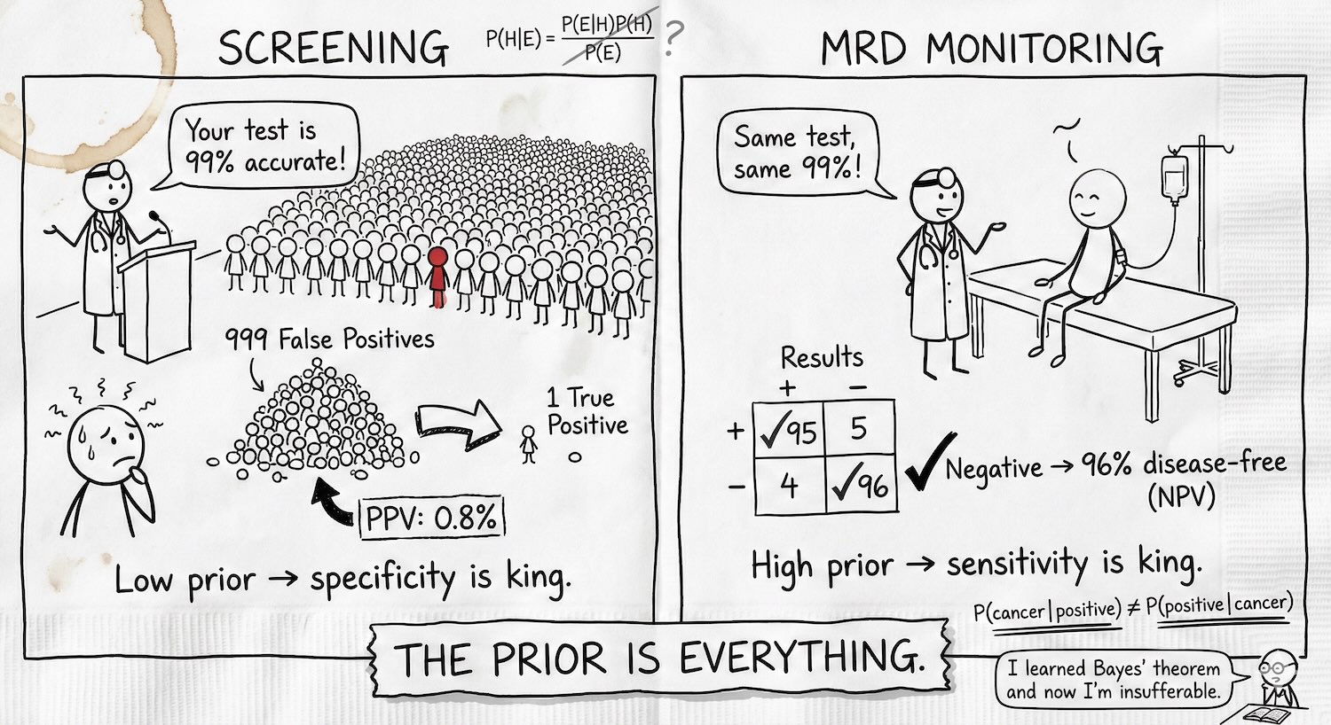TL;DR: The prior is everything. Screening healthy people (low prior)? False positives swamp true positives, specificity is king, and PPV is your metric. Monitoring a post-chemo patient (high prior)? False negatives erode trust in a clean result, sensitivity is king, and NPV is your metric. Same test, same 99% – opposite constraints, opposite failure modes. Serial testing rescues both.

Companion to the cancer diagnostics series: Part 1: The Four Pillars | Part 2: MRD | Part 3: Screening Wars. Data from OpenOnco (v. Feb 15, 2026).